Recent studies have demonstrated that spiral waves in excitable media can be generated by a phenomenon called spiral breakup (Ito & Glass, 1991; Panfilov & Holden, 1990; Gerhardt et al., 1990; Karma, 1993; Bär & Eiswirth, 1993; Panfilov & Hogeweg, 1993; Courtemanche & Winfree, 1991; Winfree, 1989). This phenomenon was discussed recently in connection with the mechanisms of cardiac fibrillation (Panfilov & Hogeweg, 1995; Winfree, 1994); spiral breakup has also been found in experiments with the Belousov-Zhabotinsky (BZ) reaction (Nagy-Ungvarai & Müller, 1994; Markus et al., 1994; Ouyang & Flesselles, 1996; Markus & Stavridis, 1994a,b). The mechanism has been discussed in several papers (Ito & Glass, 1991; Karma, 1993; Panfilov & Hogeweg, 1993). It was found to occur in models that show spatiotemporal instabilities of wave trains in 1D excitable media. The mechanism of this 1D instability is believed to be associated with the restitution properties of excitable tissue (Karma, 1994; Courtemanche et al., 1993).
However, experimental data of Markus et al. (1994) and Markus & Stavridis (1994b) suggest another possible cause of spiral breakup. In their experiments the wavefronts develop a curly shape before they break down into chaos. This curly shape is similar to the shape that is expected to occur when the wavefront is laterally unstable (Kuramoto, 1980). The mechanism of this instability is associated with a negative slope of the so-called eikonal-curvature relationship. In this paper we report on the spiral breakup occurring in a two-component FHN-model due to lateral instability.
The lateral instability of a wavefront is related to a change in the slope of the eikonal-curvature relationship. This relationship expresses the normal velocity V of a wave as a function of its curvature k. Convex and concave waves are defined by k > 0 and k < 0, respectively. It is possible to derive the following relationship for waves with a small curvature: V = V0 - Dk, where V0 is the velocity of a planar wave, and D a constant usually referred to as the effective diffusion coefficient ( Deff) (Keener, 1991). Wave instabilities occur if Deff is negative (Kuramoto, 1980). Therefore we studied the dependence of the velocity of the front on its curvature in a modified FHN-model (Panfilov & Hogeweg, 1993) in which we incorporated diffusion for both the recovery and the activator variable. We computed the value of Deff from this dependency, and by using a genetic algorithm we were able to find parameter settings for which Deff < 0. To determine the eikonal relationship, and to calculate Deff, we used fast quasi-1D computations of the eikonal equation with constant curvature of the wave (Keener, 1991). In this equation, curvature and direction of motion are pre-defined. The diffusion term is given by:
where k is the curvature and
We used the following model for an excitable medium, based on
piecewise linear `Pushchino kinetics':
with f (e) = C1e when e < e1;
f (e) = - C2e + a
when
e1 ![]() e
e ![]() e2;
f (e) = C3(e - 1) when e > e2, and
e2;
f (e) = C3(e - 1) when e > e2, and
![]() (e, g) =
(e, g) = ![]() when e < e2;
when e < e2;
![]() (e, g) =
(e, g) = ![]() when e > e2, and
when e > e2, and
![]() (e, g) =
(e, g) = ![]() when e < e1 and g < g1. To make the
function f (e) continuous,
e1 = a/(C1 + C2) and
e2 = (a + C3)/(C2 + C3). Using genetic algorithms, we found the
following basic parameter values at which we studied spiral breakup:
C1 = 43.3, C2 = 6.5, C3 = 18.3, a = 0.64, k = 9.1, g1 = 1.95,
when e < e1 and g < g1. To make the
function f (e) continuous,
e1 = a/(C1 + C2) and
e2 = (a + C3)/(C2 + C3). Using genetic algorithms, we found the
following basic parameter values at which we studied spiral breakup:
C1 = 43.3, C2 = 6.5, C3 = 18.3, a = 0.64, k = 9.1, g1 = 1.95,
![]() = 49.4,
= 49.4,
![]() = 4.4, and
= 4.4, and
![]() = 2.8. The shape of the function f (e)
specifies the fast processes. The dynamics of the recovery variable
g in the model are determined by the function
= 2.8. The shape of the function f (e)
specifies the fast processes. The dynamics of the recovery variable
g in the model are determined by the function
![]() (e, g). In
(e, g). In
![]() (e, g) the parameter
(e, g) the parameter
![]() specifies the
recovery time constant for relatively large values of g and
intermediate values of e. This region corresponds approximately to
the wavefront, waveback and to the absolute refractory
period. Similarly,
specifies the
recovery time constant for relatively large values of g and
intermediate values of e. This region corresponds approximately to
the wavefront, waveback and to the absolute refractory
period. Similarly,
![]() and
and
![]() specify the recovery time constant for large values of e, and for
small values of e and g, respectively. These regions correspond
approximately to the excited period, and to the relative refractory
period, respectively. The dynamics of g at the wavefront and the
waveback are slow, but during the excited and the relative refractory
period the dynamics are faster. The only difference between this model
and the previous model (Panfilov & Hogeweg, 1993) is that this model
incorporates diffusion of both the activator and the recovery
variable.
specify the recovery time constant for large values of e, and for
small values of e and g, respectively. These regions correspond
approximately to the excited period, and to the relative refractory
period, respectively. The dynamics of g at the wavefront and the
waveback are slow, but during the excited and the relative refractory
period the dynamics are faster. The only difference between this model
and the previous model (Panfilov & Hogeweg, 1993) is that this model
incorporates diffusion of both the activator and the recovery
variable.
For numerical computations we used the explicit Euler method with Neumann boundary conditions. To determine the velocity of waves with a fixed curvature, a wave was initiated in the linear grid, and its velocity was measured after it had become constant. This procedure was repeated for different curvatures. To initiate the first spiral in a rectangular grid we used initial data corresponding to a broken wave, the break being located in the middle of the excitable tissue.
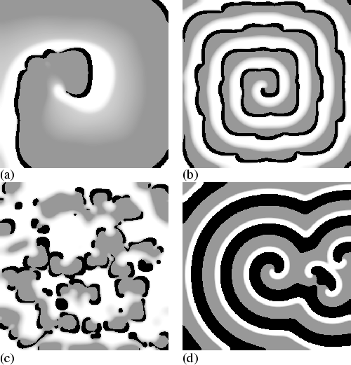
We found that spiral breakup occurred spontaneously in the excitable media at high values of Dg. Figure 2.1 shows the evolution of a spatial pattern in a medium with Dg = 2.55. The spatial pattern starts to form as soon as one spiral wave has developed. This spiral makes several rotations [Fig. 2.1(a)]. The spiral wave becomes perforated [Fig. 2.1(b)], then becomes more and more perforated, and breaks into several interacting spiral waves of different sizes [Fig. 2.1(c)]. Finally, when there is a high density of small spirals, the pattern becomes relatively stable [Fig. 2.1(d)]. These spirals are randomly distributed in space, but their centres remain in approximately fixed positions.
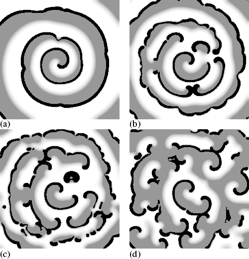 |
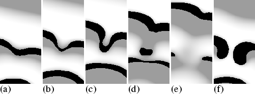
The process by which the spirals in our case were formed is shown in Fig. 2.2. The initial plane wavefront becomes unstable. In particular, part of the wavefront becomes retarded, the delay increases, and finally the wave breaks up and an excited spot is formed. This spot interacts with the following wave and creates two wave breaks, which develop into two spiral waves.
 |
The breakup that occurred in our model was not due to discrete
properties of our medium. We did computations for a wide variety of
space steps (
0.05 ![]() hs
hs ![]() 0.85). We studied the stability of
spiral breakup at various spatial and time integration steps, and
found that the patterns were similar for different degrees of
calculation precision, but the value of the parameter Dg at which
spiral breakup occurs increased as the calculation precision
increased. We found that at hs < 0.2 the shift saturated.
0.85). We studied the stability of
spiral breakup at various spatial and time integration steps, and
found that the patterns were similar for different degrees of
calculation precision, but the value of the parameter Dg at which
spiral breakup occurs increased as the calculation precision
increased. We found that at hs < 0.2 the shift saturated.
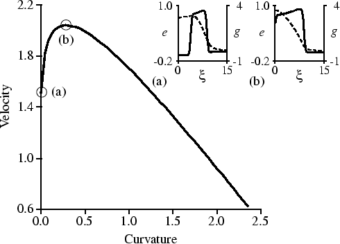
The mechanism of such breaks is due to the lateral instability of wavefronts. Figure 2.3 shows the relation between velocity V of a wave and its curvature k at the same parameter values at which we find breakup. We see that, for k < 0.3, velocity increases with increasing curvature, i.e. the wavefront here is unstable because of the lateral instability. For k > 0.3, velocity decreases with increasing curvature and wavefronts are stable again. The spiral cores are stable because they have the highest curvature.
The observation that, for small curvatures, velocity increases with curvature can be understood from a cross section through the wave. The insets of Fig. 2.3 show the values of e and g in such a cross section, for a straight and a convex wave, respectively. The velocity of a straight wave is restrained by g ahead of the wavefront. On the other hand, in the case of a convex wave the influx of g into the region before the wavefront is smaller, which leads to relatively low values of g and faster front propagation. This phenomenon is expected to be fairly general for excitable media with a high diffusion of the recovery variable (Kuramoto, 1980).
 |
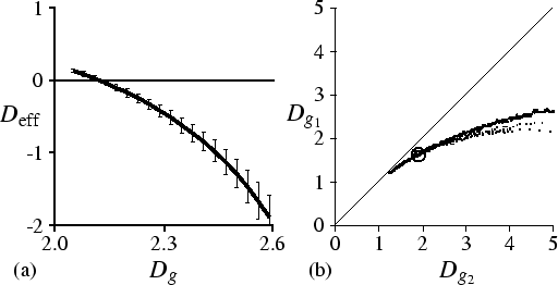
By applying regression analysis to the slope around k = 0 we
calculated the
Deff [Fig. 2.4(a)]. At
Dg ![]() 2.12,
Deff = 0. Spiral breakup is found when
Deff < - 1.2, i.e. at
2.5 < Dg < 2.6. At higher values of
Dg, propagationless patterns are found. We observed several types of
propagationless patterns with static and oscillatory behaviour,
comparable with and occurring in the same succession as the patterns
described by Ohta et al. (1989).
2.12,
Deff = 0. Spiral breakup is found when
Deff < - 1.2, i.e. at
2.5 < Dg < 2.6. At higher values of
Dg, propagationless patterns are found. We observed several types of
propagationless patterns with static and oscillatory behaviour,
comparable with and occurring in the same succession as the patterns
described by Ohta et al. (1989).
We studied the dependence of the lateral instability and spiral
breakup on the parameters of the excitable medium. We computed two
values of Dg for different parameter settings. The first
value (Dg1) is the value of Dg at which
Deff = 0,
and the second value (Dg2) is the value of Dg at which
propagationless patterns are found. The procedure was the following:
We changed the value of one parameter and, by varying the value of
Dg, we found the values Dg1 and Dg2. The results are
shown in Fig. 2.4(b). For example, for `basic
values' of parameters and numerical precision as given in the figure
caption, we get propagationless patterns at
Dg ![]() 1.98 and lateral
instability (
Deff < 0) at
Dg
1.98 and lateral
instability (
Deff < 0) at
Dg ![]() 1.68 [large open circle
in Fig. 2.4(b)]. We changed nine parameters, and
found that all nine lines of
Dg1(Dg2) are located in a small
region. The differences in Dg1 are less than 10% for
Dg2 < 3 and less than 20% for Dg2 > 3. Hence we can conclude
that lateral instability is a general property of this model. We can
also conclude that a good prediction of the occurrence of lateral
instability can be made by using the value of Dg2: For
Dg2 > 1.2 we observed lateral instabilities.
1.68 [large open circle
in Fig. 2.4(b)]. We changed nine parameters, and
found that all nine lines of
Dg1(Dg2) are located in a small
region. The differences in Dg1 are less than 10% for
Dg2 < 3 and less than 20% for Dg2 > 3. Hence we can conclude
that lateral instability is a general property of this model. We can
also conclude that a good prediction of the occurrence of lateral
instability can be made by using the value of Dg2: For
Dg2 > 1.2 we observed lateral instabilities.
 |
Low values of Dg2, at which there was no lateral instability,
were found for media with low excitability. Low excitability can be
caused by a high threshold (parameter a high), by a rapid increase
of g during the excited period (parameter k high, or parameters
![]() ,
,
![]() , or C3 low), or by
entering the refractory period at low values of g (parameter C2
low). For example, for `basic' parameter values and numerical
precision as given in Fig. 2.4(b),
Dg2 = 1.98,
while
Dg2 = 1.2 when a is changed to 0.98, or k to 17.3, or
, or C3 low), or by
entering the refractory period at low values of g (parameter C2
low). For example, for `basic' parameter values and numerical
precision as given in Fig. 2.4(b),
Dg2 = 1.98,
while
Dg2 = 1.2 when a is changed to 0.98, or k to 17.3, or
![]() to 2.7, or
to 2.7, or
![]() to 1.9, or
C3 to 5.1, or C2 to 5.1.
to 1.9, or
C3 to 5.1, or C2 to 5.1.
 |
At higher values of Dg2, the interval of values of Dg for
which we have lateral instability increases. However, lateral
instability does not necessary lead to spiral breakup for several
reasons. First, a large refractory period prevents spiral breakup,
even when the wavefront is laterally
unstable [Fig. 2.5(a)]. This is found when
![]() is high or g1 is low. In our case, if we
increased
is high or g1 is low. In our case, if we
increased
![]() to 10, or decreased g1 to 0.9,
spiral breakup disappeared. It explains why spiral breakup by lateral
instability is difficult to find in models with only one, slow,
timeconstant for the recovery variable. Secondly, a large size of the
excited region, i.e. where e > 0.6, prevents spiral
breakup [Fig. 2.5(b)]. In these cases the
instability is not strong enough to form new spirals. This is also the
case partially because the large excited region is accompanied by a
large refractory period. A large excited region is found when the
threshold is low (parameter a low), when an increase of g during
the excited period is slow (parameter k low, or parameters
to 10, or decreased g1 to 0.9,
spiral breakup disappeared. It explains why spiral breakup by lateral
instability is difficult to find in models with only one, slow,
timeconstant for the recovery variable. Secondly, a large size of the
excited region, i.e. where e > 0.6, prevents spiral
breakup [Fig. 2.5(b)]. In these cases the
instability is not strong enough to form new spirals. This is also the
case partially because the large excited region is accompanied by a
large refractory period. A large excited region is found when the
threshold is low (parameter a low), when an increase of g during
the excited period is slow (parameter k low, or parameters
![]() or C3 high), when the system enters the
refractory period at very high values of g (parameter C2 high),
or when there is a fast decrease of g behind the excited region
(parameter
or C3 high), when the system enters the
refractory period at very high values of g (parameter C2 high),
or when there is a fast decrease of g behind the excited region
(parameter
![]() low, or parameter g1 high). For
example, if we increased
low, or parameter g1 high). For
example, if we increased
![]() to 7.1, C3 to 90.0,
or C2 to 7.9, or decreased a to 0.34, k to 6.5, or
to 7.1, C3 to 90.0,
or C2 to 7.9, or decreased a to 0.34, k to 6.5, or
![]() to 2.0, breakup disappeared. Thirdly, if
to 2.0, breakup disappeared. Thirdly, if
![]() or C1 are high, the refractory period is
large, but spiral breakup is found to occur in the core of the
spiral. This eventually leads to a chaotic pattern of appearing and
disappearing spirals [Fig. 2.5(c)]. The
mechanism is a mixture of the spatiotemporal instabilities, as
described earlier
(Ito & Glass, 1991; Karma, 1993; Panfilov & Hogeweg, 1993), and the lateral
instability, as described in this paper. We found this behaviour when
we increased C1 to 250, or
or C1 are high, the refractory period is
large, but spiral breakup is found to occur in the core of the
spiral. This eventually leads to a chaotic pattern of appearing and
disappearing spirals [Fig. 2.5(c)]. The
mechanism is a mixture of the spatiotemporal instabilities, as
described earlier
(Ito & Glass, 1991; Karma, 1993; Panfilov & Hogeweg, 1993), and the lateral
instability, as described in this paper. We found this behaviour when
we increased C1 to 250, or
![]() to 100. Fourthly,
when C1 is decreased to 0.7, the spatially uniform
system (2.2) passes a point of fold bifurcation for limit
cycles. This causes the system to autocycle after an initial
stimulation. However, even before the bifurcation point (C1 < 2.3),
autocycling can be found in the spatial model. Such behaviour is
recently also described by Tsyganov et al. (1996). The autocycling
pushes aside all irregularities as caused by the lateral
instability [Fig. 2.5(d), C1 = 1.8]. Even considering
the above points, we still find breakup by lateral instability in a
fairly large region of the parameter space.
to 100. Fourthly,
when C1 is decreased to 0.7, the spatially uniform
system (2.2) passes a point of fold bifurcation for limit
cycles. This causes the system to autocycle after an initial
stimulation. However, even before the bifurcation point (C1 < 2.3),
autocycling can be found in the spatial model. Such behaviour is
recently also described by Tsyganov et al. (1996). The autocycling
pushes aside all irregularities as caused by the lateral
instability [Fig. 2.5(d), C1 = 1.8]. Even considering
the above points, we still find breakup by lateral instability in a
fairly large region of the parameter space.
The wave patterns obtained in our computations are similar to those obtained in the experiments performed by Markus et al. (1994) and Markus & Stavridis (1994a,b). The mechanisms of the instabilities are also similar. In the light-sensitive BZ reaction the slope of the eikonal-curvature dependence was found to be both positive and humped (Markus & Stavridis, 1994a), just as in our computations. However, it is not clear which mechanisms generate the positive slope in the BZ reaction. In our model the positive slope occurs because of the large diffusion coefficient of the inhibitor. In the light-sensitive BZ reaction the diffusions of chemical species are of the same order of magnitude. However, in the case of the BZ reaction, an increase in the concentration inhibitor Br- is determined by its diffusion coefficient multiplied by the rate constant of its auto-catalysis. It is known that light enhances the production of Br-, and it may be this enhanced increase in the Br- concentration which leads to the curly wavefronts and spiral breakups (Markus & Stavridis, 1994a).
The mechanism of instability that causes the spiral breakup described in this paper is fundamentally different from the 1D instability which is responsible for the earlier observations of spiral breakup (Ito & Glass, 1991; Karma, 1993; Panfilov & Hogeweg, 1993). First, it is a pure two-dimensional mechanism, and it has no counterpart in 1D systems. Secondly, not only wave trains, but also solitary waves show this instability.
Although lateral instabilities of wavefronts have not been described earlier in models for excitable media, they have been found in bistable systems (Hagberg & Meron, 1994; Horváth et al., 1993). Horváth et al. (1993) found an unstable wavefront but no spiral breakup. Hagberg & Meron (1994) showed that lateral instability made turbulence possible through Ising-Bloch front bifurcations. An analytical study of other types of spatial instabilities of wave trains was reported by Kessler & Levine (1990).
We expect the phenomenon of spiral breakup by lateral instability to be not uncommon in excitable media and that it is probably easy to find comparable behaviour in other models of excitable media with non-fixed time-scales for the recovery variable.

